# notepad or the R scripting window and it should line up
# This program is a little more complicated than the previous ones,and some of
# the topics may be a little out of the scope of this class, but if you
# are interested and don't understand something let me know
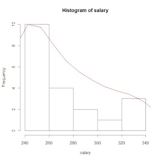
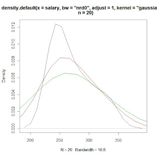
# example plots from Part 2 of the program using sample salary data:
# histogram of salary data with gaussian KDE plot

# KDE plots of salary data with varying bandwidth selections using the 'adjust'
# option

# PROGRAM NAME: KDE_R
# DATE: 6/18/2010
# AUTHOR : MATT BOGARD
# PURPOSE: EXAMPLE OF KERNAL DENSITY ESTIMATES IN R
# DATA USED: SIMULATED WITHIN SCRIPT
# PACKAGES: lattice Hmisc
# OUTPUT FILE: "C:\Documents and Settings\wkuuser\My Documents\TOOLS AND REFERENCES\R References"
# UPDATES:
#
#
# COMMENTS: GIVE A BASIC UNDERSTANDING OF THE density() FUNCTION IN R
# AND BANDWIDTH, KERNAL SELECTION, AND PLOTTING
#
# REFERENCES: ADAPTED FROM
# http://ise.tamu.edu/metrology/Group%20Seminars/Kernel_Density_Estimation_2008JUN27_2.pdf
#
# CONTENTS: PART1 EXAMPLES USING CODE GENERATED NORMALLY DISTRIBUTED DATA
# PART2 EXAMPLES USING SAMPLE DATA
#---------------------------------------------------------------#
# PART1 EXAMPLES USING CODE GENERATED NORMALLY DISTRIBUTED DATA
#---------------------------------------------------------------#
x <- seq(-4, 4, 0.01) y <- dnorm(x, mean=0, sd=1 # create x,y data set that is exactly normal
rn <- rnorm(1000, mean=0, sd=1 # create a set of random normal values
# plot the density of the random numbers you just generated
# let the bandwidth = nrd0 "rule of thub" h= .9*A*n*exp(-1.5), A = min{s,IQR/1.34}
# select the gaussian kernal using 1000 points (which you just generated)
plot(density(x=rn, bw="nrd0", kernel="gaussian", n=1000), col=5) # gaussian is default
lines(x, y) # plot the exactly normal data set you created earlier to compare
# plot a series of KDE plots with varying bandwitdth using 'width='option
# When this option is specified instead of 'bw',and is a number, the density
# function bandwidth is set to a kernel dependent multiple of 'width'
for(w in 1:3)
lines(density(x=rn, width=w, kernel="gaussian", n=1000), col=w+1)
# what if we change the kernal
# first close the graphics window to start over
# look at varius bandwidths using a kernal other than gaussian
# KDE otpions:
# gaussian rectangular triangular
# biweight cosine optcosine"
# epanechnikov
plot(density(x=rn, bw="nrd0", kernel="rectangular", n=1000), col=1)
for(w in 1:3)
lines(density(x=rn, width=w, kernel="rectangular", n=1000), col=w+1)
# or to just look at various densities in one plot
# using a lines statment specifying the specific kernal
plot(density(x=rn, bw="nrd0", kernel="gaussian", n=1000), col=1)
lines(density(x=rn, bw="nrd0", kernel="rectangular", n=1000), col=2)
lines(density(x=rn, bw="nrd0", kernel="triangular", n=1000), col=3)
lines(density(x=rn, bw="nrd0", kernel="epanechnikov", n=1000), col=4)
lines(density(x=rn, bw="nrd0", kernel="biweight", n=1000), col=5)
lines(density(x=rn, bw="nrd0", kernel="cosine", n=1000), col=6)
lines(density(x=rn, bw="nrd0", kernel="optcosine", n=1000), col=7)
# or to just look at various densities in one plot
# using a lines statment specifying the specific kernal
plot(density(x=rn, bw="nrd0", kernel="gaussian", n=1000), col=1)
# note if you want the default gaussian, it does not have to be specified
plot(density(x=rn, bw="nrd0", n=1000), col=1)
#-----------------------------------#
# PART2 EXAMPLES USING SAMPLE DATA
#-----------------------------------#
# load salary data
salary<-c(240,240,240,240,240,240,240,240,255,255,265,265,280,280,290,300,305,325,330,340)
print(salary)
library(Hmisc) # load for describe function
describe(salary) # general stats
library(lattice) # load lattice package for histogram graphics
hs <- hist(salary) # plot histogram and store data
print(hs)
# create a kde of salary data (gaussian)and store it as dens
dens <- density(x=salary, bw="nrd0", n=20)
print(dens)
rs <- max(hs$counts/max(dens$y)) # create scaling factor for plotting the density
lines(dens$x, dens$y*rs, col=2) # plot density over histogram using lines statment
# compare this to just plotting the non-rescaled density over the histogram
lines(density(x=salary, bw="nrd0", n=20),col=3) # green line barely shows up
# also, compare to just plotting the estimated density for the sample
# data in a separate plot
plot(density(x=salary, bw="nrd0", n=20)) # or equivalently
plot(dens, col=3)
# now that we understand the various ways we can plot a specified KDE
# we can apply the tools used in part 1 to look at the effects of
# various bandwidths and kernal choices - first close the graphing window
# what if we change the kernal
# first close the graphics window to start over
# look at varius KDEs
# KDE otpions:
# gaussian rectangular triangular
# biweight cosine optcosine"
# epanechnikov
# look at various densities in one plot
# using a lines statment specifying the specific kernal
plot(density(x=salary, bw="nrd0", kernel="gaussian", n=20), col=1)
lines(density(x=salary, bw="nrd0", kernel="rectangular", n=20), col=2)
lines(density(x=salary, bw="nrd0", kernel="triangular", n=20), col=3)
lines(density(x=salary, bw="nrd0", kernel="epanechnikov", n=20), col=4)
lines(density(x=salary, bw="nrd0", kernel="biweight", n=20), col=5)
lines(density(x=salary, bw="nrd0", kernel="cosine", n=20), col=6)
lines(density(x=salary, bw="nrd0", kernel="optcosine", n=20), col=7)
# what if we don't specify a bandwidth (clear graphics window)
# what is the default density
plot(density(x=salary, bw="nrd0", kernel="gaussian", n=20), col=1)
lines(density(x=salary, kernel="gaussian", n=20), col=2)# nrd0 appears to be default
# what if we change the default
# nrd (a variation of nrd0)
# ucv (unbiased cross validation)
# bcv (cross validation)
lines(density(x=salary, bw="ucv", kernel="gaussian", n=20), col=2)
lines(density(x=salary, bw="bcv", kernel="gaussian", n=20), col=3)
lines(density(x=salary, bw="nrd", kernel="gaussian", n=20), col=4)
# use print option to see how the bw value changes with each method
print(density(x=salary, bw="nrd0", kernel="gaussian", n=20))
# look at the differences in calculated
# bandwidth and plots with the adjust option
for(w in 1:3)
print(density(x=salary, bw="nrd0", adjust=w, kernel="gaussian", n=20))
plot(density(x=salary, bw="nrd0",adjust=1, kernel="gaussian", n=20), col=1)
lines(density(x=salary, bw="nrd0",adjust=2,kernel="gaussian", n=20), col=2)
lines(density(x=salary, bw="nrd0",adjust=3,kernel="gaussian", n=20), col=3)
