The Constutution, Public Choice and Democracy

There are certainly differences between the ways that markets allocate resources ( using prices which reflect trade-offs based on the knowledge and preferences of millions of individuals) vs government (which allocates resources using command and control based on the more limited knowledge and preferences of a few voters, elected officials, or appointed bureaucrats).

The economic analysis of political institutions represents a sub field of economics referred to as 'Public Choice Economics.' The following link will take you to an article 'The Public Choice Revolution', Regulation Fall 2004.

This article summarizes some of the major findings from the field of public choice. The article discusses among many things, why do we need government, and what are the tradeoffs between tyranny (or Leviathan ) and anarchy.

"Once it is admitted that the state is necessary, positive public choice analyzes how it assumes its missions of allocative efficiency and redistribution. Normative public choice tries to identify institutions conducive to individuals getting from the state what they want without being exploited by it."

Another section looks at the analysis of voting. It discusses problems with using voting to allocate resources, such as cycling and the median voter theorem. It also looks at issues related to special interests, bureaucracies, and the role of representative government in democratic systems.

"In our democracies, voters do not decide most issues directly. In some instances, they vote for representatives who reach decisions in parliamentary assemblies or committees. In other instances, they elect representatives who hire bureaucrats to make decisions. The complexity of the system and the incentives of its actors do not necessarily make collective choices more representative of the citizens’ preferences."

Particularly the article looks at how more government with a larger budget leads to more power for special interests:

"Interest groups will engage in what public choice theorists call “rent seeking,” i.e., the search for redistributive benefits at the expense of others. The larger the state and the more benefits it can confer, the more rent-seeking will occur. “The entire federal budget,” writes Mueller, “can be viewed as a gigantic rent up for grabs for those who can exert the most political muscle.”

The moral of the public choice story is that democracy and governments are not perfect. When we have issues with market outcomes and we are thinking about new regulations or government spending to correct those problems, public choice analysis offers a guide. Public choice analysis implies that we have to question which system will provide the best information and incentives to act on that information to achieve the results that we want. The U.S. Consittution with its separation of powers and the specifically enumerated powers in Article 1 Section 8 provides a framework for achieving this balance. The democratic process itself offers no guarantee that the decision will be the best solution to our problems.

Markets and Knowledge- with Applications to Disaster Relief

I Pencil -The actual essay starts on page 4 within the document (actually page 8 in the pdf) This discusses the role that prices play in conveying knowledge and directing and organizing behavior in society- often described as a ‘spontaneous order.’


Economics has many applications outside of what you may stereotypically have in mind. Besides giving insight into how to run a business, economic principles apply to other areas of human behavior, like for instance, disaster response:

The Use of Knowledge in Disaster Relief Management


Government’s Response to Hurricane Katrina: A public choice analysis


Again, these are really upper level applications of basic principles of economics. Don’t feel overwhelmed by the material. Just scan through and try to get a general idea. What we will cover in class will be much more basic. However, these are great examples of applications of the principles we will talk about in class.

Using R

Many people that are involved in data analysis may have one software package that they prefer to use, but may never have heard of R, or even thought about trying something new. R is a statistical programming language with a command line interface that is becoming more and more popular every day. If you are used to a point and click interface (like SPSS or Excel for example) the learning curve for R may be quite steep but well worth the effort. If you are already familiar with a programming language, like SAS for instance, (SPSS also has a command line interface) the switch to R may not be that difficult but could be very rewarding. In fact there is a free version of a reference available entitled ‘R for SAS and SPSS Users’ that I found very helpful getting started.

How I use R

I often use SAS for data management, recoding, merging and sub-setting data sets, and cleaning and formatting data. I’m getting better at doing some of these things in R but I just have more experience in SAS. I first became interested in using R for spatial lag models and geographically weighted regression, which requires the construction of spatial weights matrices. (These techniques aren't as straight forward if at all possible in SAS). I've also used R for data visualization, data mining/machine learning, as well as social network analysis. I give my students the option to use R in the statistics course I teach and I have had several pursue it. And most recently, I have become acquainted with SAS IML Studio, which is a product that will better enable me to integrate some of my SAS related projects with some of the powerful tools R provides.

How can you use R?

Google’s Chief Economist Hal Varian uses R . His paper Predicting the Present with Google Trends is a great example of how R can be used for prediction, and is loaded with R code and graphics. Facebook uses R as well:

“Facebook’s Data Team used R in 2007 to answer two questions about new users: (i) which data points predict whether a user will stay? and (ii) if they stay, which data points predict how active they’ll be after three months?” (Link- how Google and Facebook are using r by Michael E. Driscoll at Dataspora.com)

The New York Times recently did a feature on R entitled ‘Data Analysts Captivated by R’ where industry leaders explain why and how they use R.

“Companies like Google and Pfizer say they use the software for just about anything they can. Google, for example, taps R for help understanding trends in ad pricing and for illuminating patterns in the search data it collects. Pfizer has created customized packages for R…Companies as diverse as Google, Pfizer, Merck, Bank of America, the InterContinental Hotels Group and Shell use it.”

The article goes on to discuss the proliferate and diverse packages offered by R:

“One package, called BiodiversityR, offers a graphical interface aimed at making calculations of environmental trends easier. Another package, called Emu, analyzes speech patterns, while GenABEL is used to study the human genome. The financial services community has demonstrated a particular affinity for R; dozens of packages exist for derivatives analysis alone.”

In a recent issue of Forbes (Power in the Numbers by Quentin Hardy May 2010) R is discussed as a powerful analysis tool as well as its potential to revolutionize business, markets, and government:

‘Using an R package originally for ecological science, a human rights group called Benetech was able to establish a pattern of genocide in Guatemala. A baseball fan in West Virginia used another R package to predict when pitchers would get tired, winning himself a job with the Tampa Bay Rays. An R promoter in San Francisco, Michael Driscoll, used it to prove that you are seven times as likely to change cell phone providers the month after a friend does. Now he uses it for the pricing and placement of Internet ads, looking at 100,000 variables a second”

“Nie posits that statisticians can act as watchdogs for the common man, helping people find new ways to unite and escape top-down manipulation from governments, media or big business...It's a great power equalizer, a Magna Carta for the devolution of analytic rights… "

The proprietary adaptation of R, Revolution R was recently discussed on Fox Business; you can see the interview here.

A good way to get a look at what researchers are doing with R would be to review presentation topics at a past UseR conference, from 2008:


Andrew Gelman, Bayesian generalized linear models and an appropriate default prior

Michael Höhle, Modelling and surveillance of infectious diseases - or why there is an R in SARS

E. James Harner, Dajie Luo, Jun Tan, JavaStat: a Java-based R Front-end

Robert Ferstl, Josef Hayden, Hedging interest rate risk with the dynamic Nelson/Siegel model

Jacob Michaelson, Andreas Beyer, Random Forests for eQTL Analysis: A Performance Comparison

Graham J. WilliamsDeploying , Data Mining in Government - Experiences With R/Rattle

Jing Hua Zhao, Qihua Tan, Shengxu Li, Jian'an LuanSome, Perspectives of Graphical Methods for Genetic Data

Who else uses R?

A review of past participant lists from UseR also gives you a pretty good idea about companies that are using R. Past participants includes:

Merril Lynch, Merck Research Laboratories , Siemens AG,, BASF SE, Astra Zeneca, Bayer CropScience, Novartis Pharma, AT&T Labs, Bell Labs, Bank of Canada, Credit Suisse, Max Planck Institute, US Naval Academy, Harvard, Vanderbilt University + many universities.

UCLA has great online resources for R and Stanford offers a course called Elements of Statistical Learning which utilizes a textbook with the same title that heavily references R code.


Downloading and using R

For more information about R and to download it to try it yourself, the place to start is the R Project website: http://www.r-project.org/

A few other great references for R can be found here:

Quick R (Statistics Guide)- http://www.statmethods.net/index.html

Revolution Analytics- (Blog) - http://blog.revolutionanalytics.com/

http://www.r-bloggers.com/

Facebook- R Bloggers Group
Statistical Computing with R: A Tutorial (Illinois State University) –

http://math.illinoisstate.edu/dhkim/rstuff/rtutor.html(UCLA R Class Notes) -great example code for getting started with R –
http://www.ats.ucla.edu/stat/R/notes/Using R for Introductory Statistics (John Verzani) - http://cran.r-project.org/doc/contrib/Verzani-SimpleR.pdf


References:

Changing the Face of Analytics. Fox Business Network via YouTube: http://www.youtube.com/watch?v=4nOMhTBuXl8&feature=youtube_gdata

Data Analysts Captivated by R’s Power. New York Times. January 6, 2009.

Driscoll, Michael E. How Google and Facebook Are Using R. Dataspora Blog. February 19, 2009. http://dataspora.com/blog/predictive-analytics-using-r/

Hardy, Quentin. Power in Numbers. Forbes Magazine. May 24,2010.

Hastie, Tibshirani, and Friedman. The Elements of Statistical Learning. Second Edition. February 2009. http://www-stat.stanford.edu/~tibs/ElemStatLearn/

Hyunyoung Choi and Hal Varian. Predicting the Present with Google Trends. Google Inc.
Draft Date April 10, 2009. http://static.googleusercontent.com/external_content/untrusted_dlcp/www.google.com/en/us/googleblogs/pdfs/google_predicting_the_present.pdf

R 4stats.com: http://rforsasandspssusers.com/

The R Project: http://www.r-project.org/

UCLA Resources to Help You Learn and Use R: http://www.ats.ucla.edu/stat/R/

Kernal Density Plots

# When viewing this post the code looks messy, but just copy and paste into
# notepad or the R scripting window and it should line up

# This program is a little more complicated than the previous ones,and some of
# the topics may be a little out of the scope of this class, but if you
# are interested and don't understand something let me know


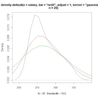
# example plots from Part 2 of the program using sample salary data:

# histogram of salary data with gaussian KDE plot




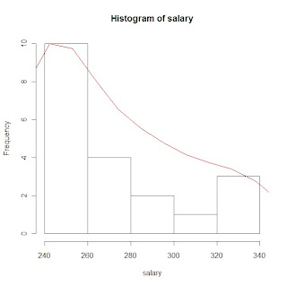
# KDE plots of salary data with varying bandwidth selections using the 'adjust'
# option







# PROGRAM NAME: KDE_R
# DATE: 6/18/2010
# AUTHOR : MATT BOGARD
# PURPOSE: EXAMPLE OF KERNAL DENSITY ESTIMATES IN R
# DATA USED: SIMULATED WITHIN SCRIPT
# PACKAGES: lattice Hmisc
# OUTPUT FILE: "C:\Documents and Settings\wkuuser\My Documents\TOOLS AND REFERENCES\R References"
# UPDATES:
#
#
# COMMENTS: GIVE A BASIC UNDERSTANDING OF THE density() FUNCTION IN R
# AND BANDWIDTH, KERNAL SELECTION, AND PLOTTING
#
# REFERENCES: ADAPTED FROM
# http://ise.tamu.edu/metrology/Group%20Seminars/Kernel_Density_Estimation_2008JUN27_2.pdf
#
# CONTENTS: PART1 EXAMPLES USING CODE GENERATED NORMALLY DISTRIBUTED DATA
# PART2 EXAMPLES USING SAMPLE DATA

#---------------------------------------------------------------#
# PART1 EXAMPLES USING CODE GENERATED NORMALLY DISTRIBUTED DATA
#---------------------------------------------------------------#

x <- seq(-4, 4, 0.01) y <- dnorm(x, mean=0, sd=1 # create x,y data set that is exactly normal

rn <- rnorm(1000, mean=0, sd=1 # create a set of random normal values

# plot the density of the random numbers you just generated
# let the bandwidth = nrd0 "rule of thub" h= .9*A*n*exp(-1.5), A = min{s,IQR/1.34}
# select the gaussian kernal using 1000 points (which you just generated)



plot(density(x=rn, bw="nrd0", kernel="gaussian", n=1000), col=5) # gaussian is default

lines(x, y) # plot the exactly normal data set you created earlier to compare



# plot a series of KDE plots with varying bandwitdth using 'width='option
# When this option is specified instead of 'bw',and is a number, the density
# function bandwidth is set to a kernel dependent multiple of 'width'

for(w in 1:3)
lines(density(x=rn, width=w, kernel="gaussian", n=1000), col=w+1)


# what if we change the kernal
# first close the graphics window to start over
# look at varius bandwidths using a kernal other than gaussian

# KDE otpions:
# gaussian rectangular triangular
# biweight cosine optcosine"
# epanechnikov


plot(density(x=rn, bw="nrd0", kernel="rectangular", n=1000), col=1)
for(w in 1:3)
lines(density(x=rn, width=w, kernel="rectangular", n=1000), col=w+1)


# or to just look at various densities in one plot
# using a lines statment specifying the specific kernal

plot(density(x=rn, bw="nrd0", kernel="gaussian", n=1000), col=1)
lines(density(x=rn, bw="nrd0", kernel="rectangular", n=1000), col=2)
lines(density(x=rn, bw="nrd0", kernel="triangular", n=1000), col=3)
lines(density(x=rn, bw="nrd0", kernel="epanechnikov", n=1000), col=4)
lines(density(x=rn, bw="nrd0", kernel="biweight", n=1000), col=5)
lines(density(x=rn, bw="nrd0", kernel="cosine", n=1000), col=6)
lines(density(x=rn, bw="nrd0", kernel="optcosine", n=1000), col=7)

# or to just look at various densities in one plot
# using a lines statment specifying the specific kernal

plot(density(x=rn, bw="nrd0", kernel="gaussian", n=1000), col=1)

# note if you want the default gaussian, it does not have to be specified

plot(density(x=rn, bw="nrd0", n=1000), col=1)


#-----------------------------------#
# PART2 EXAMPLES USING SAMPLE DATA
#-----------------------------------#

# load salary data

salary<-c(240,240,240,240,240,240,240,240,255,255,265,265,280,280,290,300,305,325,330,340)
print(salary)

library(Hmisc) # load for describe function
describe(salary) # general stats

library(lattice) # load lattice package for histogram graphics
hs <- hist(salary) # plot histogram and store data
print(hs)

# create a kde of salary data (gaussian)and store it as dens

dens <- density(x=salary, bw="nrd0", n=20)
print(dens)


rs <- max(hs$counts/max(dens$y)) # create scaling factor for plotting the density
lines(dens$x, dens$y*rs, col=2) # plot density over histogram using lines statment

# compare this to just plotting the non-rescaled density over the histogram

lines(density(x=salary, bw="nrd0", n=20),col=3) # green line barely shows up

# also, compare to just plotting the estimated density for the sample
# data in a separate plot


plot(density(x=salary, bw="nrd0", n=20)) # or equivalently
plot(dens, col=3)

# now that we understand the various ways we can plot a specified KDE
# we can apply the tools used in part 1 to look at the effects of
# various bandwidths and kernal choices - first close the graphing window

# what if we change the kernal
# first close the graphics window to start over
# look at varius KDEs

# KDE otpions:
# gaussian rectangular triangular
# biweight cosine optcosine"
# epanechnikov


# look at various densities in one plot
# using a lines statment specifying the specific kernal

plot(density(x=salary, bw="nrd0", kernel="gaussian", n=20), col=1)
lines(density(x=salary, bw="nrd0", kernel="rectangular", n=20), col=2)
lines(density(x=salary, bw="nrd0", kernel="triangular", n=20), col=3)
lines(density(x=salary, bw="nrd0", kernel="epanechnikov", n=20), col=4)
lines(density(x=salary, bw="nrd0", kernel="biweight", n=20), col=5)
lines(density(x=salary, bw="nrd0", kernel="cosine", n=20), col=6)
lines(density(x=salary, bw="nrd0", kernel="optcosine", n=20), col=7)

# what if we don't specify a bandwidth (clear graphics window)
# what is the default density

plot(density(x=salary, bw="nrd0", kernel="gaussian", n=20), col=1)
lines(density(x=salary, kernel="gaussian", n=20), col=2)# nrd0 appears to be default

# what if we change the default
# nrd (a variation of nrd0)
# ucv (unbiased cross validation)
# bcv (cross validation)

lines(density(x=salary, bw="ucv", kernel="gaussian", n=20), col=2)
lines(density(x=salary, bw="bcv", kernel="gaussian", n=20), col=3)
lines(density(x=salary, bw="nrd", kernel="gaussian", n=20), col=4)

# use print option to see how the bw value changes with each method

print(density(x=salary, bw="nrd0", kernel="gaussian", n=20))

# look at the differences in calculated
# bandwidth and plots with the adjust option

for(w in 1:3)
print(density(x=salary, bw="nrd0", adjust=w, kernel="gaussian", n=20))


plot(density(x=salary, bw="nrd0",adjust=1, kernel="gaussian", n=20), col=1)
lines(density(x=salary, bw="nrd0",adjust=2,kernel="gaussian", n=20), col=2)
lines(density(x=salary, bw="nrd0",adjust=3,kernel="gaussian", n=20), col=3)

Inference, Hypothesis Testing, & Regression

Inference: the exercise of providing information about the population based on information contained in the sample

Type 1 Error: rejecting a true null hypothesis
- the probabability of rejecting a true null hypothesis ( or the probability of a type 1 error) is equal to alpha or 'α' This is also the same as the level of significance in a hypothesis test.

Type II Error: failing to reject, or loosely speaking, 'accepting' the null hypthesis when it is false
-the probability of a type II error =beta or β

Power: the probability of rejecting the null hypothesis when it is false. (1-β)

Regression Model: describes how the dependent variable (y) is related to the independent variable (x), also known as the least squares line.

y = b0 + b1*x

This is derived by the process of least squares, which gives the value for the slope (b1) and the intercept (bo) that minimizes the sum of the squared deviations between the observed values of the dependent variable (Y) and the estimated values of the dependent variable (Y*).

Co-efficient of determination(R-squared) = SSR/SST -> gives the proportion of total variation explained by the regression model. Larger values indicate that the sample data are closer to the least squares line, or a stronger linear relationship exists.

Standard Normal Distribution & Z-values

############################################
# Below is R code for plotting normal distributions - illustrating
# the changes in the distribution when standard deviation changes.
# -selected graphics are imbedded below
#
# Also calculates area under the normal curve for given Z
#
# Finally plots 3-D bivariate normal density
#
#############################################



# PROGRAM NAME: NORMAL_PLOT_R
#
# ECON 206
#
# ORIGINAL SOURCE: The Standard Normal Distribution in R:
# http://msenux.redwoods.edu/math/R/StandardNormal.php
#
#
#
#


#PLOT NORMAL DENSISTY

x=seq(-4,4,length=200)
y=dnorm(x,mean=0,sd=1)
plot(x,y,type="l",lwd=2,col="red")

#######################################





###################################





# INCREASE THE STANDARD DEVIATION

x=seq(-4,4,length=200)
y=dnorm(x,mean=0,sd=2.5)
plot(x,y,type="l",lwd=2,col="red")


#####################################



####################################

# DECREASE THE STANDARD DEVIATION

x=seq(-4,4,length=200)
y=dnorm(x,mean=0,sd=.5)
plot(x,y,type="l",lwd=2,col="red")

# CALCULATING AREA FOR GIVEN Z-VALUES

# RECALL, FOR THE STANDARD NORMAL DISTRIBUTION THE MEAN = 0 AND
# THE STANDARD DEVIATION = 1
# THE pnorm FUNCTION GIVES THE PROBABILITY FOR THE AREA TO THE LEFT
# OF THE SPECIFIED Z-VALUE ( THE FIRST VALUE ENTERED IN THE FUNCTION)
# THE OUTPUT SHOULD MATCH WHAT YOU GET FROM THE NORMAL TABLE IN YOUR BOOK
# OR THE HANDOUT I SENT YOU

pnorm(0,mean=0, sd=1) # Z =0

pnorm(1,mean=0, sd=1) # Z <= 1

pnorm(1.55, mean=0, sd=1) # Z<=1.55

pnorm(1.645, mean=0, sd=1) # Z<= 1.645


# LETS LOOK AT A BIVARIATE NORMAL
# DISTRIBUTION


# first simulate a bivariate normal sample

library(MASS)

bivn <- mvrnorm(1000, mu = c(0, 0), Sigma = matrix(c(1, 0, 0, 1), 2))

# now we do a kernel density estimate

bivn.kde <- kde2d(bivn[,1], bivn[,2], n = 100)

# now plot your results

contour(bivn.kde)
image(bivn.kde)

persp(bivn.kde, phi = 45, theta = 30)


# fancy contour with image

image(bivn.kde); contour(bivn.kde, add = T)

# fancy perspective

persp(bivn.kde, phi = 45, theta = 30, shade = .1, border = NA)

###############################################

Regression Demo